Hassaan Saleem

In this post, I will explain what Renormalization Group (RG) flow is. I will assume the knowledge of the basics of QFT for this post.

The idea of an RG flow is intimately related to the idea of effective field theories (EFTs). An EFT is a theory that makes predictions upto some energy scale (called μ) but after this energy scale, it breaks down. The length scale corresponding to the energy scale μ is called μ^-1 and the EFT makes predictions for distances larger than μ^-1.

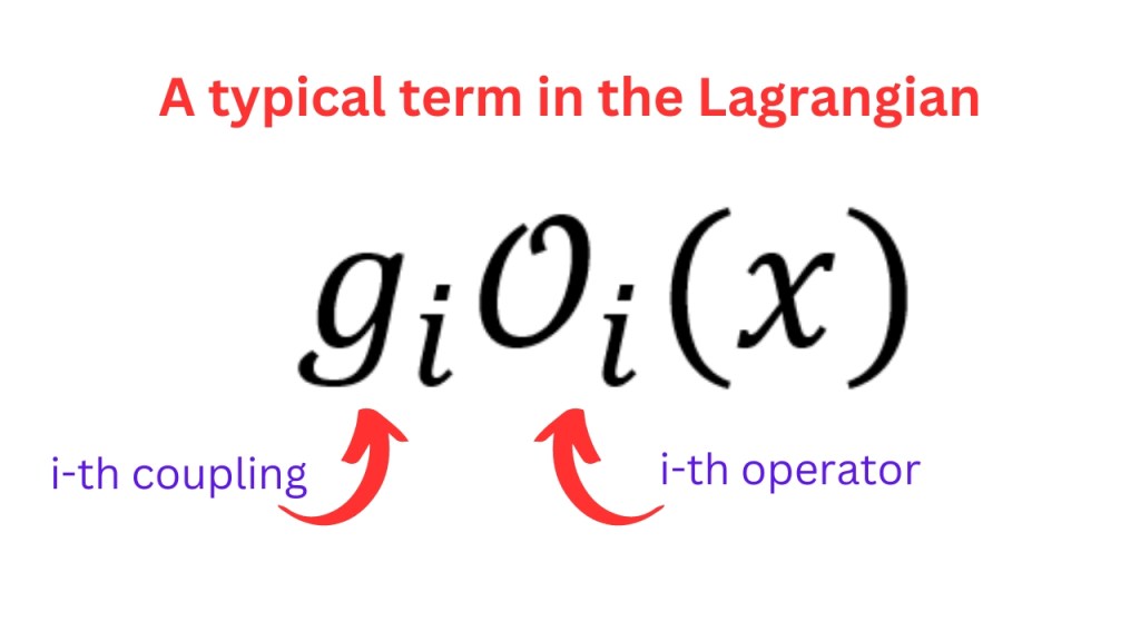
In EFTs, we can include all the possible terms in the lagrangian, without worrying if these terms will give divergent results for arbitrarily high energies, because we don’t want to make predictions for arbitrarily high energies. For each of the terms in the lagrangian, we have a coupling that multiplies an operator. Let’s call these couplings g_i.

An EFT describes the physics of energy scales less than μ in terms of the degrees of freedom (DOFs) at scales less than μ. The DOFs at higher energies just contribute to determining the couplings for this EFT (masses also come under the rubrik of couplings in this context). Therefore, the couplings g_i can depend on where the cutoff μ is. Hence, we write the couplings as g_i(μ).

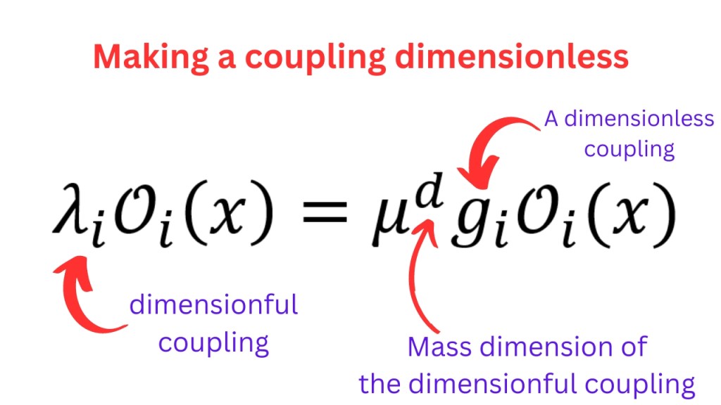
We will require that all of these couplings are dimensionless. If there is a a coupling that has some mass dimension, we can write it as a dimensionless coupling, multiplied by some power of μ. Therefore, it is consistent to take all g_is as dimensionless.

We can now make a theory space T where the coordinates are these couplings g_i. Since there are potentially infinite number of terms that we can put into a lagrangian, there is potentially an infinite number of couplings and thus, T can be inifnite dimensional. Each point in this space represents a field theory.

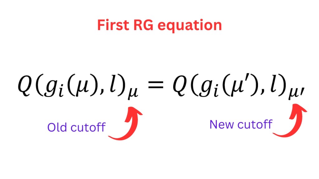
Now, the main idea of the RG is flow is that if there is a physical quantity, that is being calculated at a length scale L (with corresponding energy scale E), which is larger than μ^-1, and this quantity depends on the couplings g_i(μ) (let’s call this quantity Q(g_i(μ),L)_μ) then this quantity shouldn’t change if we change the cutoff μ (to some μ’), while still keeping μ larger than E. Please note that the couplings g_i(μ) will change as the cutoff changes, but the physical quantities don’t change. This translates to the following equation.

There is another equation that we can work out. Suppose that we start from the quantity Q(g_i(μ),L)_μ and bring down the cutoff to μ/s (with s>1) while E still being smaller than μ/s. This quantity should now become Q(g_i(μ/s),L)_μ/s. Now, if we do a scale transformation, scaling all energies by s (which implies that we rescale all lengths by 1/s and anything with a mass dimension D scales as s^D), the quantity should become s^d_Q Q(g_i(μ/s),L/s)_μ where d_Q is the mass dimension of the quantity Q. This implies that we have the following equation.

This equation tells us that (at the fixed cutoff μ) the physical quantity Q calculated at length scale sL with couplings g_i(μ) is the same (upto the s^d_Q) when calculated at the shorter length scale L but with couplings g_i(μ/s) i.e. changing the length scale from L to sL has the same effect as keeping the length scale at L but changing the coupling from g_i(μ) to g_i(μ/s).

This is one of the key ideas of RG flow i.e. couplings change with the energy scale at which we want to make predictions (which gives a ‘flow’ in the theory space T). In terms of the theory space, the cutoff μ is a parameter on the flow line that connects a theory at infinite μ (called the UV theory) and a theory at μ=0 (called the IR theory).

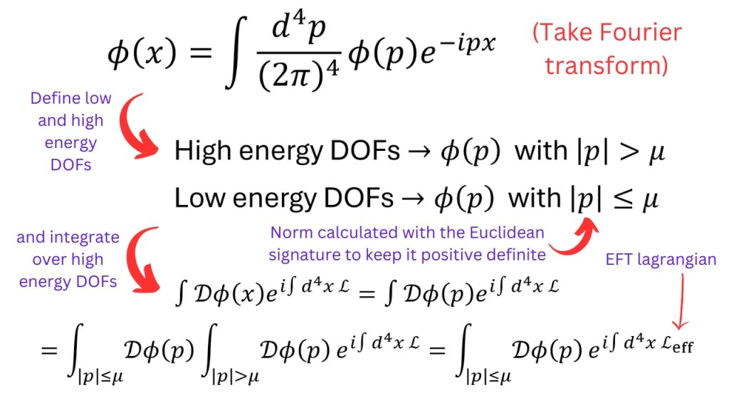
I want to emphasize here that the direction of the RG flow is from a high energy cutoff to a low energy cutoff. This is because if you want to make EFT of a theory that makes sensible predictions to all energies (called a UV complete theory), we get rid off the higher energy DOFs by integrating them out. Remember that in a path integral, we have to integrate over all possible field configurations. If we divide the DOFs of our field into high energy and low energy modes, and integrate over only the high energy modes, the lagrangian that appears in the path integral changes and become the effective lagrangian of the EFT. This also changes the couplings in the lagrangian, as discussed before. Doing this integration sends us from higher cutoffs to lower cutoffs and thus, this is the natural direction of the RG flow.

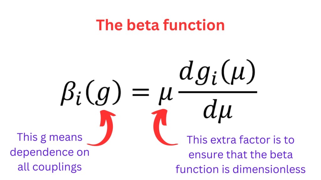
Since the couplings change with the cutoff μ, we can calculate the derivative of the coupling g_i(μ) with respect to the cutoff. This idea leads to defining a quantity called the beta function β_i(g₁,g₂,…) where I have made it manifest that beta function of the ith coupling g_i(μ) can depend on all the other couplings as well. It means that the beta function is a function defined over the theory space T.

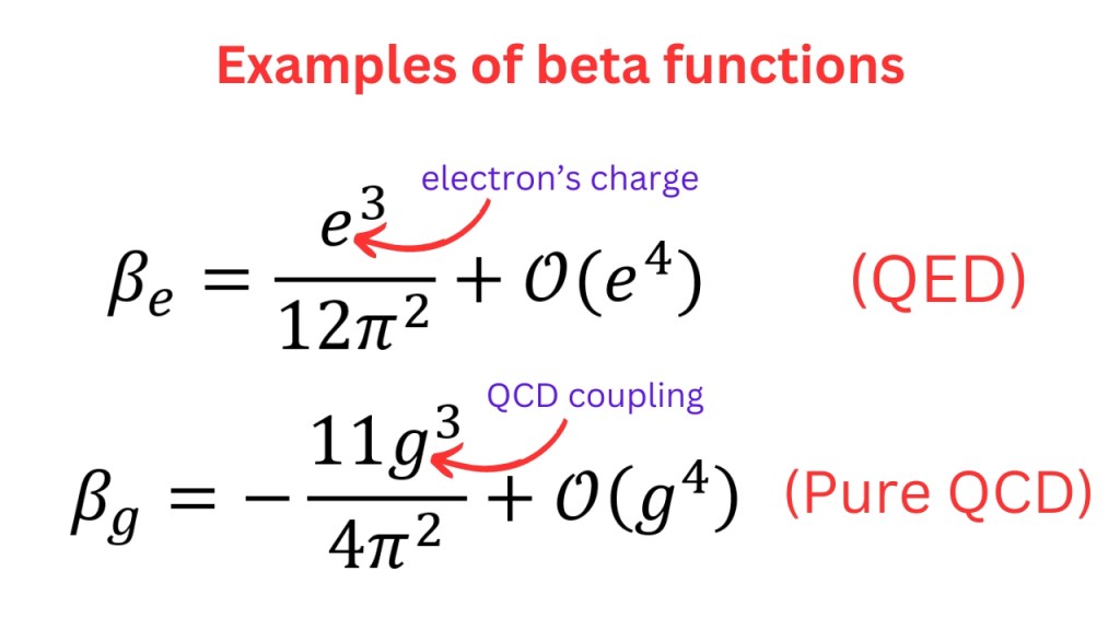
Now, we can see that if the beta function of a quantity is positive, it means that as μ increases, the coupling increases. Remember that increasing μ means goint to higher cutoffs (or short distances). This is the case with QED. If instead the beta function is negative, the coupling decreases with increasing μ. This behaviour is called asymptotic freedom. This is the case with QCD.

What if the beta function is zero? It would mean that the coupling is not changing with the cutoff μ. Any point in T where beta function is zero is called a fixed point. Fixed points are theories of course. These theories have scale symmetry (i.e. the coupling doesn’t change with the energy scale) and these fixed points are conformal field theories (CFTs).

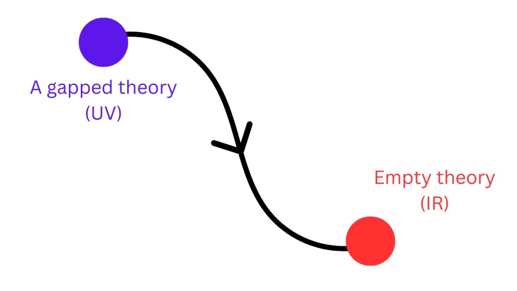
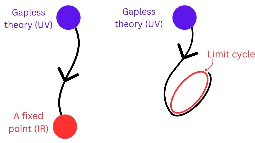
When the RG flow starts from some UV theory, it can either go to an empty theory, or some nontrivial fixed point. If the UV theory has no massless particles, then eventually, the cutoff will go below the mass of the lightest particle and thus, we will not have any more propagating degrees of freedom. Therefore we will have an empty theory. A theory with no massless particles is called a gapped theory (also called a “mass gap” theory). A gapped UV theory will flow to an empty theory.

Now consider a UV theory with some massless particle (such theories are called gapless theories). This theory can’t flow to an empty theory because it will have at least one propagating DOF (i.e. the massless particle) no matter how small μ becomes. Thus, this UV theory has to flow to something else. Such UV theories mostly flow to a fixed point (sometimes they flow to structures called limit cycles but we won’t talk about them).

Now, in T, consider the region around a fixed point. We can try to model this region by perturbing the CFT that the fixed point represents by adding a term to the lagrangian of the CFT that consists of some operator in that CFT. What will happen if we try different operators for this perturbation?

One possibility is that such a perturbation flows back into the fixed point. If this happens, the operator that produced this perturbation is called an irrelevant operator. Another possibility is that such a perturbation flows away from this fixed point. In this case, the operator that produced this perturbation is called a relevant operator.

For readers familiar with CFT, I can mention that an operator is relevant if the scaling dimension of that operator is smaller than the dimension of the spacetime in which the CFT is defined. If the scaling dimension is larger than the spacetime dimension, the operator is irrelevant. It turns out that the number of relevant operators in a CFT is much smaller than the number of irrelevant operators.

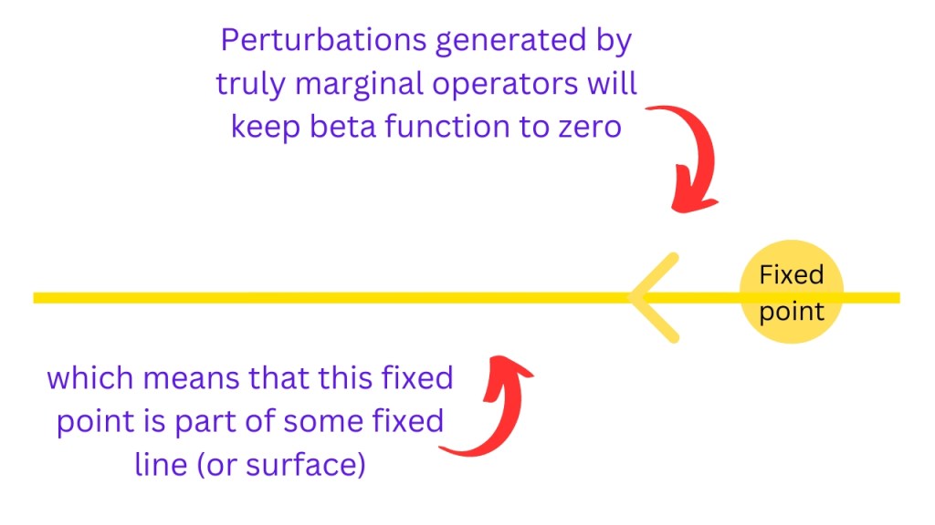
Is there any other possibility? Suppose that we perturb a fixed point by some operator, and for all of this small perturbation, the beta function stays exactly zero. It would mean that the fixed point that we were considering isn’t an isolated fixed point, but a point in some fixed line or fixed surface and the perturbation is keeping us on this line or surface. Operators that produce these kind of perturbations are called truly marginal operators.

For those readers who are familiar with RG flows, I want to mention that I am not going into the nitty gritties of marginally relevant and marginally irrrelevant operators.

The remaining blogpost will be a little deviod of details but will contain a summary of useful results. If you start at a fixed point and perturb this CFT (let’s call it the UV CFT) with a relevant operator, you can flow to another CFT (IR CFT). There are some known results about the RG flows between two CFTs.

One such result holds in 2 dimensional CFTs (i.e. 2D CFTs) and it is called the Zamolodchikov c-theorem. There is a property of 2D CFTs called the central charge which is used to classify CFTs as well. The c-theorem says that if the CFT is unitary, then the central charge of the UV CFT is bigger than the central charge of the IR CFT. This is a very powerful result that allows us to constrain the possible RG flows.

There is a similar result for 4D CFTs called the a-theorem (by Cardy, Komargodski and Schwimmer) which says that a quantity called the “Euler anomaly coefficient” decreases along RG flows. In addition, for 2D CFTs that live on a spacetime with a boundary, there is a theorem called the g-theorem which that the g-function (which is roughly the entropy of the boundary) decreases. However, this result comes with a lot of caveats.

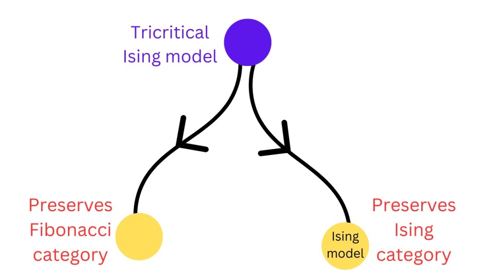
Lastly, there are symmetries that can be preserved by some RG flows and broken by other flows. These symmetries include the usual group symmetries and some exotic non-invertible symmetries (also called categorical symmetries). For example, there is a 2D CFT called the tricritical Ising model. It has a categorical symmetry that is made of two categories i.e. the Ising category and the Fibonacci category. It has two RG flows to two different CFTs. One RG flow preserves the Ising category symmetry and the other RG flow preserves the Fibonacci symmetry. So, symmetries (includng categorical symmetries) can be a good way to identity RG flows between CFTs.